Run Statistical Ensembles with Inductiva

In this guide, you’ll learn how to run statistical ensembles in parallel using Inductiva, so you can turn any parameter sweep or distribution into dozens (or hundreds!) of simultaneous simulations. We’ll demonstrate with a classic 2D Ising-model Metropolis Monte Carlo in R, but this workflow works with any function or simulation script that takes parameters and outputs results.

Rather than looping through parameters one at a time, Inductiva lets you launch a group of machines, run tasks concurrently, and collect outputs automatically. This means you can get ensemble results in minutes instead of hours.

What You'll Accomplish

1. Package your simulation – Convert your simulation code (in this case, an R script) to accept parameters from the command line and output results to CSV.
2. Define your ensemble – Specify a list or distribution of parameters (e.g., temperatures, seeds, reaction rates) to explore.
3. Launch cloud machines – Allocate as many workers as ensemble tasks.
4. Dispatch parallel jobs – SSend each parameter set as an individual job. Inductiva manages queuing, scaling, retries, and logging.
5. Visualize ensemble output – Plot summary statistics like means, variances, or distributions using a few lines of code.

Need a refresher on the Ising model? See 2D Ising model on Wikipedia

For more on the the 2D Ising-model details, see the 2D Ising model description

Prepare Your Ensemble Script

First, wrap your simulation logic in a script that:

• Reads one or more parameter values from the command line
• Runs your script over those parameters
• Writes its results to an output file (in this case a CSV)

Here’s an example for run_ising_model.R. The example takes a list of “temperature” values, but you can swap in any numeric parameter (reaction rate, seed, boundary condition, etc.).

Rscript run_ising_model.R \
  --temps "1.5,2.0,2.5" \
  --grid-size 100 \
  --n-sweeps 20000 \
  --burn-in 2000 \
  --thin 20 \
  --output results.csv

💡 Pro tip: Any script that reads --param-list and writes a CSV with columns like ParamValue, Sweep, Output1, Output2, … can slot into this Inductiva workflow.

Launching your ensemble with Inductiva

Suppose you want to examine how minor perturbations around a temperature affect the Ising model. With Inductiva, you can sample from a normal distribution around the base temperature, run all simulations in parallel, and collect the full set of results — without managing infrastructure.

In this section we will explore step by step how you can create a python script with Inductiva to easily create the ensemble.

1. Setup and Configuration

Import the necessary libraries, point to your R script folder (INPUT_DIR), and pick where to save results (RESULTS_DIR). Define the base temperatures, the number of samples around each, and the Normal‐sampling spread (sigma).

import os
import numpy as np
import pandas as pd
import matplotlib.pyplot as plt
import inductiva

INPUT_DIR = "./input"
RESULTS_DIR = "./results"
OUTPUT_ROOT = "inductiva_output"
PROJECT_NAME = "temperature_ensemble_3_0"

BASE_TEMPERATURE = 3.0
NUM_SAMPLES = 50
TEMPERATURE_SIGMA = 0.05
RNG_SEED = 123

NSWEEPS = 10000
BURNIN = 1000
N_SPINS = 100
THIN = 10

# Ensure results directory exists
os.makedirs(RESULTS_DIR, exist_ok=True)

2. Sample Temperatures from a Normal Distribution around T0

For a base temperature T₀, draw n_samples points from 𝒩(T₀, σ²). That gives you one “central” run at T₀, plus a spread of values around it.

np.random.seed(RNG_SEED)
sampled_temps = sorted(
    np.random.normal(loc=BASE_TEMPERATURE,
                     scale=TEMPERATURE_SIGMA,
                     size=NUM_SAMPLES))

3. Spin Up the Cloud Machines

Next, calculate the total number of runs (one for each T₀ plus all its samples), and use the Inductiva API to spin up that many machines. We’ll use an ElasticMachineGroup, which automatically grows to match task load. You can control the maximum number of machines via the max_machines parameter.

all_temps = [BASE_TEMPERATURE] + sampled_temps
max_machines = len(all_temps)

machine_group = inductiva.resources.ElasticMachineGroup(
    machine_type="c2-standard-8",
    spot=True,
    min_machines=1,
    max_machines=max_machines,
)

# Use the R docker container simulator
sim = inductiva.simulators.CustomImage(container_image="docker://r-base:latest")

# Define a project for the current tasks
project = inductiva.projects.Project(project_name)

4. Submit Every Temperature as Its Own Task

Loop over each sample of T₀, round each temperature, build the Rscript command, and submit. You can also attach metadata for easy information retrieval later.

for temp in all_temps:
    t_val = round(temp, 3)
    output_filename = f"ising_T0_{BASE_TEMPERATURE:.1f}_samp{t_val:.3f}.csv"

    command = (f'Rscript run_ising_model.R '
               f'--N {N_SPINS} --temps "{t_val}" '
               f'--nsweeps {NSWEEPS} --burnin {BURNIN} --thin {THIN} '
               f'--output {output_filename}')

    task = simulator.run(
        input_dir=INPUT_DIR,
        on=machine_group,
        commands=[command],
        project=PROJECT_NAME,
    )

    task.set_metadata({
        "base_temperature": str(BASE_TEMPERATURE),
        "sample_temperature": str(t_val),
        "output_file": output_filename,
        "task_id": task.id,
    })

    print(f"Submitted: T₀={BASE_TEMPERATURE} temp={t_val} → {output_filename}")

5. Wait for Completion and Download Results

Now that every task was submitted we can wait until every task in the project finishes. Then, pull down all their CSV outputs into the default inductiva_output/<PROJECT_NAME>/ folder.

# Wait for all tasks in the project to end
project.wait()

# Download all outputs from the project
project.download_outputs()

At this point, you’ll have one CSV per temperature value, ready to merge and analyze.

Visualize Ensemble Results

Finally, pull in every CSV produced around our base temperature, stack them into one DataFrame, and compute at each sweep:

1. ⟨M⟩ (mean magnetization) across all sampled runs
2. Lower (2.5%) and upper (97.5%) percentiles of M

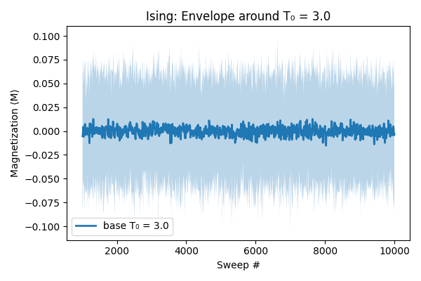
Plotting the mean curve with this confidence band shows the central behavior and the spread across simulations.

We then plot the mean curve across sweep numbers and shade the region between those percentiles. This shaded area, called the envelope, captures the spread or uncertainty in the Monte Carlo realizations around T₀, providing both a central trend and a visual indication of variability across runs.

# Gather all metadata from the project
all_tasks = project.get_tasks()
metadata_list = [task.get_metadata() for task in all_tasks]

csv_paths = []
for meta in metadata_list:
    if meta["base_temperature"] != str(BASE_TEMPERATURE):
        continue
    tid = meta["task_id"]
    fname = meta["output_file"]
    path = os.path.join(OUTPUT_ROOT, PROJECT_NAME, tid, "outputs", fname)
    csv_paths.append(path)

# read & concatenate
df = pd.concat((pd.read_csv(p) for p in csv_paths), ignore_index=True)

# compute mean ± 95% CI of M by sweep
summary = df.groupby("sweep")["M"].agg(
    M_mean="mean",
    M_lo=lambda x: x.quantile(0.025),
    M_hi=lambda x: x.quantile(0.975)).reset_index()

# plot envelope
plt.figure(figsize=(6, 4))
plt.plot(summary["sweep"],
         summary["M_mean"],
         lw=2,
         label=f"Base T₀ = {BASE_TEMPERATURE}")

plt.fill_between(summary["sweep"], summary["M_lo"], summary["M_hi"], alpha=0.3)
plt.xlabel("Sweep #")
plt.ylabel("Magnetization ⟨M⟩")
plt.title(f"Ising: Envelope around T₀ = {BASE_TEMPERATURE}")
plt.legend()
plt.tight_layout()

out_png = os.path.join(RESULTS_DIR, f"magnetization_T0_{BASE_TEMPERATURE}.png")
plt.savefig(out_png)
plt.close()

print(f"✔ Saved envelope plot for T₀={BASE_TEMPERATURE} → {out_png}")

The image below shows the result of this ensemble run:

Wrapping Up

And that wraps up our end-to-end workflow:

1. Prepared the R-based Monte Carlo script
2. Orchestrated parallel runs via Python + Inductiva
3. Collected output from every run
4. Merged and visualized the ensemble results

You can now observe how magnetization evolves across sweeps for each base temperature and its nearby samples.