Run a Temporal Boundary Layer with Stable Stratification Case

This tutorial was written by Pedro Costa (TU Delft) in collaboration with the Inductiva Team

Special thanks to Dr. Baptiste Hardy (TU Delft) for his support in devising this temporal boundary layer setup

The numerical simulation of a temporally evolving, stably stratified boundary layer offers a clear computational sandbox for exploring fundamental fluid dynamics relevant to atmospheric wind flows.

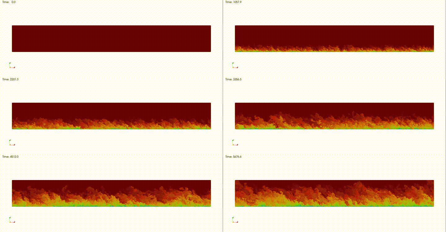
Understanding boundary layer physics is critical in atmospheric modeling because wind characteristics, turbulence structure, and mixing processes strongly depend on boundary layer dynamics. The temporal boundary layer (TBL) setup is useful for understanding boundary layer turbulence at high Reynolds numbers typical of atmospheric flows. The higher the Reynolds number of a wind flow boundary layer, the more "locally parallel" the flow is. The TBL flow consists of a moving bottom wall with constant velocity, with turbulence being entrained to the flow vertically and parallel to the wall. This asymptotically approximates the development of windflow over a surface as it approaches a parallel state, allowing simple interpretation of turbulent processes.

Stability plays a crucial role in altering boundary layer dynamics 1. To better understand its effects, let's examine the types of stratification conditions:

• Neutral stratification (no vertical temperature gradient) provides a baseline scenario where temperature doesn't affect the wind turbulence dynamics.

• In stable stratification, temperature decreases with the height (that is, denser air near the surface and lighter air above), and buoyancy suppresses vertical movements, reducing turbulent mixing, and overall boundary layer growth.

• Conversely, in unstable stratification (cooler air above warmer air), buoyancy amplifies vertical motions, enhancing turbulence and thickening the boundary layer.

(not animated here)

Simulating these different stratification conditions provides insight into how buoyancy and turbulence interact to shape the wind boundary layer.

This tutorial focuses on simulating stable stratification, where warmer air overlies cooler air, as it closely reflects common atmospheric conditions - particularly at night due to radiative cooling of the land surface or during stable weather patterns.

1 Nieuwstadt, Frans T.M. "The turbulent structure of the stable, nocturnal boundary layer." Journal of Atmospheric Sciences 41.14 (1984): 2202–2216.

Simulate Stable Stratification

Prerequisites

To run this use case, begin by creating the input.nml with the following contents:

&dns
ng(1:3) = 576, 576, 384
l(1:3) = 150, 75, 80
gtype = 2, gr = 2.
cfl = 0.95, dtmax = 1.e5
visci = 1000.
inivel = 'tbl'
is_wallturb = F
nstep = 40000, time_max = 2000., tw_max = 0.1
stop_type(1:3) = T, F, F
restart = F, is_overwrite_save = T, nsaves_max = 0
icheck = 10, iout0d = 100, iout1d = 100, iout2d = 200, iout3d = 20000, isave = 5000
cbcvel(0:1,1:3,1) = 'P','P',  'P','P',  'D','N'
cbcvel(0:1,1:3,2) = 'P','P',  'P','P',  'D','N'
cbcvel(0:1,1:3,3) = 'P','P',  'P','P',  'D','D'
cbcpre(0:1,1:3)   = 'P','P',  'P','P',  'N','N'
bcvel(0:1,1:3,1) =  0.,0.,   0.,0.,   1.,0.
bcvel(0:1,1:3,2) =  0.,0.,   0.,0.,   0.,0.
bcvel(0:1,1:3,3) =  0.,0.,   0.,0.,   0.,0.
bcpre(0:1,1:3)   =  0.,0.,   0.,0.,   0.,0.
bforce(1:3) = 0., 0., 0.
is_forced(1:3) = F, F, F
velf(1:3) = 0., 0., 0.
gacc(1:3) = 0., 0., -1.
nscal = 1
dims(1:2) = 0, 0, ipencil_axis = 3
/

&scalar
iniscal(:)             = 'tbl'
alphai(:)              = 710.  ! = Pr/nu = 500 * 0.71
beta                   = -0.004 ! = Gr/Re_D^2, Gr = 1e3, Re_D=500
cbcscal(0:1,1:3,:)     = 'P'  ,'P' ,  'P','P',  'D','N'
bcscal(0:1,1:3,:)      =  0.,0. ,   0.,0. ,   1.,0.
is_sforced(:)          = F
scalf(:)               = 0.
is_boussinesq_buoyancy = T
/

&cudecomp
cudecomp_t_comm_backend = 0, cudecomp_is_t_enable_nccl = T, cudecomp_is_t_enable_nvshmem = T
cudecomp_h_comm_backend = 0, cudecomp_is_h_enable_nccl = T, cudecomp_is_h_enable_nvshmem = T
/

&numerics
is_impdiff = F, is_impdiff_1d = T
is_poisson_pcr_tdma = F
/

&other_options
is_debug = T, is_timing = T
/

To simulate neutral or unstable stratification instead of the stable case, simply modify the beta parameter in the configuration file:

• Set beta = 0 for neutral stratification
• Set beta = 0.004 for unstable stratification

Running the Simulation

Here is the code required to run the simulation using the Inductiva API:

"""CaNS example."""
import inductiva

# Allocate cloud machine on Google Cloud Platform
cloud_machine = inductiva.resources.MachineGroup( \
        provider="GCP",
        machine_type="a2-highgpu-2g",
        zone="europe-west4-b",
        data_disk_gb=100,
        spot=True)

# Initialize the Simulator
cans = inductiva.simulators.CaNS(\
    version="3.0.0")

# Run simulation
task = cans.run(input_dir="/Path/to/SimulationFiles",
    sim_config_filename="input.nml",
    on=cloud_machine)

# Wait for the simulation to finish and download the results
task.wait()
cloud_machine.terminate()

task.download_outputs()

task.print_summary()

Note: Setting spot=True enables the use of spot machines, which are available at substantial discounts. However, your simulation may be interrupted if the cloud provider reclaims the machine.

When the simulation is complete, we terminate the machine, download the results and print a summary of the simulation as shown below.

Task status: Success

Timeline:
    Waiting for Input         at 08/06, 15:06:42      0.758 s
    In Queue                  at 08/06, 15:06:43      65.05 s
    Preparing to Compute      at 08/06, 15:07:48      17.726 s
    In Progress               at 08/06, 15:08:06      10029.364 s
        ├> 1.07 s          mkdir -p data
        └> 10028.036 s     /opt/openmpi/4.1.6/bin/mpirun --np 2 --use-hwthread-cpus cans input.nml
    Finalizing                at 08/06, 17:55:15      640.376 s
    Success                   at 08/06, 18:05:56

Data:
    Size of zipped output:    19.72 GB
    Size of unzipped output:  22.20 GB
    Number of output files:   2639

Total estimated cost (US$): 8.87 US$
    Estimated computation cost (US$): 8.86 US$
    Task orchestration fee (US$): 0.010 US$

Note: A per-run orchestration fee (0.010 US$) applies to tasks run from 01 Dec 2025, in addition to the computation costs.
Learn more about costs at: https://inductiva.ai/guides/how-it-works/basics/how-much-does-it-cost

As you can see in the "In Progress" line, the part of the timeline that represents the actual execution of the simulation, the core computation time of this simulation was approximately 2 hours and 47 minutes.

Scaling Up the Simulation

One of the key advantages of using Inductiva is the ease with which you can scale your simulations to larger, more powerful machines with minimal changes to your code. Scaling up simply involves updating the machine_type parameter when allocating the cloud machine.

To explore detailed results, visit our Benchmarks page.