Why wait for cluster time when others are publishing? Run your simulations now and stay ahead.
Run the e-H scattering Tutorial
In this tutorial, we’ll model the scattering of an electron wavepacket off a hydrogen atom using Octopus through the Inductiva API.
This is the same e-H scattering example featured in the official Octopus tutorials.
To simplify and speedup the simulation, we’ll work in one dimension (1D), which also makes it easier to visualize key physical quantities. The setup can be easily adapted to perform a full three-dimensional (3D) simulation of a hydrogen atom.
Prerequisites
Create a folder named SimulationFiles and place the following files inside it:
Your SimulationFiles folder should look like this:
SimulationFiles/
├── e-h-scat.inp
├── gs.inp
└── plot.gp
Running the Simulation
Here is the code required to run an Octopus simulation using the Inductiva API:
"""Octopus example"""
import inductiva

# Allocate cloud machine on Google Cloud Platform
cloud_machine = inductiva.resources.MachineGroup( \
    provider="GCP",
    machine_type="c2d-highcpu-4",
    spot=True)

# Initialize the Simulator
octopus = inductiva.simulators.Octopus( \
    version="16.1")

commands = [
    "mv gs.inp inp",
    "octopus",
    "mv inp gs.inp",
    "mv e-h-scat.inp inp",
    "octopus",
    "mv inp e-h-scat.inp",
    # Generate plots
    "gnuplot plot.gp",
    # Generate gif from plots
    "convert -delay 20 -loop 0 potential_*.png scattering.gif"
]

# Run simulation
task = octopus.run( \
    input_dir="/Path/to/SimulationFiles",
    commands=commands,
    on=cloud_machine)

task.wait()
cloud_machine.terminate()

task.download_outputs()

task.print_summary()
Note: Setting
spot=Trueenables the use of spot machines, which are available at substantial discounts. However, your simulation may be interrupted if the cloud provider reclaims the machine.
This example consists of four main steps:
- Ground-State Calculation:
We begin by running
octopuswith the input fileqs.inp. This performs the ground-state calculation and generates therestart/gsdirectory, which stores the wavefunctions and other data required for the next stage. - Time-Dependent Simulation:
Next, we run
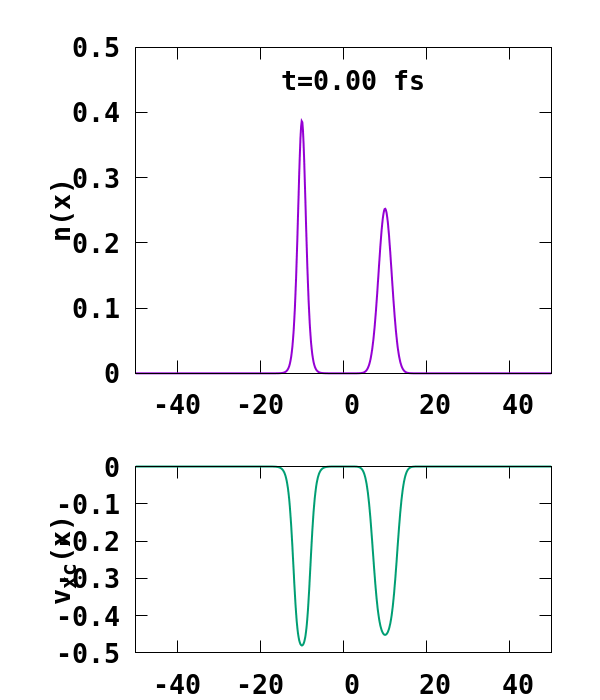
octopuswith the input filee-h-scat.inp. This performs a time-dependent (TD) real-time propagation calculation for a one-dimensional hydrogen-like system using a soft-Coulomb potential. The system starts from scratch and models a single hydrogen atom located at position -10, with an extra electron added, leading to a negatively charged system. - Generating Plots:
In this step, we run a
Gnuplotscript that generates time-resolved plots of the electron density and exchange-correlation potential from the simulation. It creates PNG images at selected time steps, illustrating how the wavepacket and potential evolve during the real-time propagation. - Generating GIFs:
Finally, we run the
convertcommand to compile the generated plots into a GIF, creating an animated visualization of the simulation.
When you run the Python script above, the simulation is executed on a cloud machine of type c2d-highcpu-4, which provides
4 virtual CPUs. For larger or more compute-intensive simulations, consider adjusting the machine_type parameter to
select a machine with more virtual CPUs and increased memory capacity. You can explore the full range of available machines here.
After the simulation completes, the machine is terminated automatically, the results are downloaded, and a summary of the simulation is printed, as shown below.
Task status: Success

Timeline:
    Waiting for Input         at 15/07, 11:21:09      0.743 s
    In Queue                  at 15/07, 11:21:10      41.361 s
    Preparing to Compute      at 15/07, 11:21:52      4.081 s
    In Progress               at 15/07, 11:21:56      685.099 s
        ├> 1.148 s         mv gs.inp inp
        ├> 2.087 s         octopus
        ├> 1.084 s         mv inp gs.inp
        ├> 1.092 s         mv e-h-scat.inp inp
        ├> 472.522 s       octopus
        ├> 1.074 s         mv inp e-h-scat.inp
        ├> 7.09 s          gnuplot plot.gp
        └> 198.277 s       convert -delay 20 -loop 0 potential_*.png scattering.gif
    Finalizing                at 15/07, 11:33:21      1.349 s
    Success                   at 15/07, 11:33:22

Data:
    Size of zipped output:    38.64 MB
    Size of unzipped output:  102.43 MB
    Number of output files:   2777

Total estimated cost (US$): 0.0145 US$
    Estimated computation cost (US$): 0.0045 US$
    Task orchestration fee (US$): 0.010 US$

Note: A per-run orchestration fee (0.010 US$) applies to tasks run from 01 Dec 2025, in addition to the computation costs.
Learn more about costs at: https://inductiva.ai/guides/basics/how-much-does-it-cost
As you can see in the "In Progress" line, the part of the timeline that represents the actual execution of the simulation, the core computation time of this simulation was approximately 11 minutes and 25 seconds.
Testing Different Machines
This simulation is relatively small, using a one-dimensional setup with a single atom. Consequently, increasing the number of vCPUs has little to no impact on performance. To investigate potential speedups, we tested configurations with 4 and 8 vCPUs across several machine series, comparing performance across hardware generations.
| Machine Type | Execution Time | Estimated Cost (USD) |
|---|---|---|
| c2d-highcpu-4 | 11 min, 25s | 0.0045 |
| c2d-highcpu-8 | 11 min, 22s | 0.0082 |
| c3d-highcpu-4 | 11 min, 15s | 0.0079 |
| c3d-highcpu-8 | 11 min, 11s | 0.0150 |
| c4-highcpu-4 | 6 min, 51s | 0.0092 |
| c4-highcpu-8 | 7 min, 14s | 0.0190 |
These results confirm that increasing the number of vCPUs has minimal effect on performance for this small simulation, with
runtimes nearly identical between 4 and 8 vCPUs. The newer c4-highcpu machines complete the task significantly faster than the c2d and c3d series, though at a higher cost. Among the options tested, c2d-highcpu-4 is the most cost-effective, while c4-highcpu-4 delivers the best performance. This highlights the limited benefit of scaling CPU count for this particular simulation.