From your laptop to large-scale simulations with five lines of Python.
Flow Around a Circular Cylinder 🌀
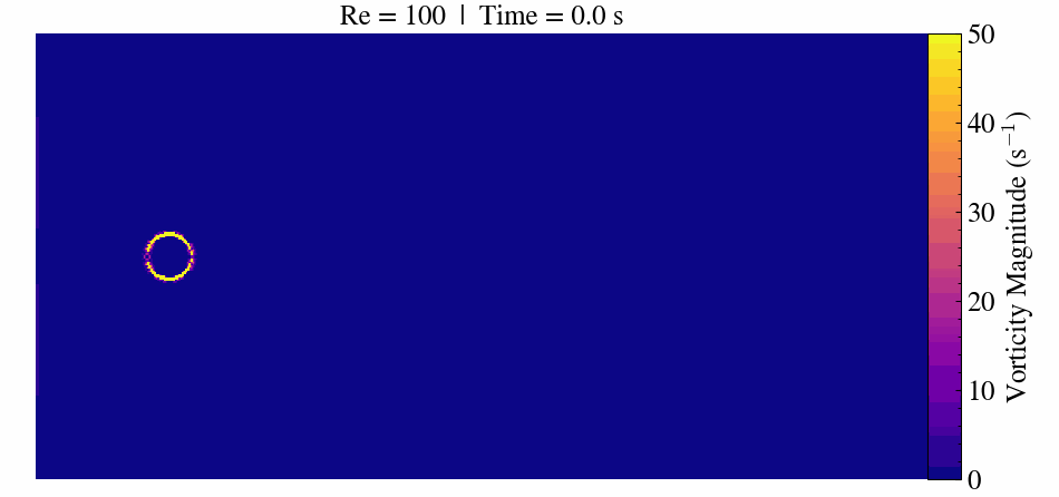
This tutorial will simulate a flow over a cylinder case using AMR-Wind. This classic fluid dynamics problem reveals the changes in flow behavior depending on the Reynolds number (Re).
We will cover the ib_cylinder_Re_300 use case from the test files folder of the AMR-Wind GitHub repository.
To demonstrate Inductiva's scalability, we will run the same simulation on cloud machines with varying levels of computational power.

Case Description
The flow around a circular cylinder has been extensively studied because it captures fundamental fluid dynamics phenomena. At very low Reynolds numbers (Re < 5), the flow remains steady and symmetric. As Re increases, the flow begins to separate and forms steady recirculation zones.
When the Reynolds number surpasses approximately 47, the flow transitions to an unsteady regime. Here, periodic vortex shedding develops, creating the characteristic von Kármán vortex street.
At Re = 300, the flow becomes fully three-dimensional and unsteady. This makes it a popular benchmark for validating CFD solvers, immersed boundary methods, and mesh refinement strategies.
Run the Circular Cylinder Case
Prerequisites
Download the required files here.
Case Modifications
To support a more compute-intensive workload than the original configuration, we made the following changes to the input file (ib_cylinder_Re_300.inp):
- Increased
time.max_stepfrom 20 to 2000 - This extension avoids the skew caused by the slower initial warm-up iterations and ensures a longer runtime, enabling a more accurate and meaningful performance comparison across machines. - Increased
time.plot_intervalfrom 10 to 2000 - Since intermediate results are not of interest in this case, we set the plotting frequency equal to the maximum number of time steps. This ensures that only the final result is written, reducing unnecessary output. - Increased
amr.n_cellfrom 64 64 16 to 256 256 64 - The mesh resolution was increased by a factor of four in each dimension to fully utilize the GPU. The original case was too small to reflect representative performance. With refinement zones included, the final mesh contains nearly 16 million cells.
Running the Simulation
Below is the code required to run the simulation using the Inductiva API.
In this example, we use a g2-standard-12 cloud machine, equipped with 12 virtual CPUs (vCPUs) and an NVIDIA L4 GPU.
"""AMR-Wind example."""
import inductiva

# Allocate cloud machine on Google Cloud Platform
cloud_machine = inductiva.resources.MachineGroup( \
    provider="GCP",
    machine_type="g2-standard-12",
    spot=True)

# Initialize the Simulator
amr_wind = inductiva.simulators.AmrWind(\
    version="3.4.1")

# Run simulation
task = amr_wind.run(input_dir="/Path/to/flow-cylinder-case",
    n_vcpus=1, # number of GPUs
    sim_config_filename="ib_cylinder_Re_300.inp",
    on=cloud_machine)

# Wait for the simulation to finish and download the results
task.wait()
cloud_machine.terminate()

task.download_outputs()

task.print_summary()
Note: Setting
spot=Trueenables the use of spot machines, which are available at substantial discounts. However, your simulation may be interrupted if the cloud provider reclaims the machine.
When the simulation is complete, we terminate the machine, download the results and print a summary of the simulation as shown below.
Task status: Success

Timeline:
    Waiting for Input         at 17/09, 14:13:24      0.868 s
    In Queue                  at 17/09, 14:13:24      48.062 s
    Preparing to Compute      at 17/09, 14:14:13      22.299 s
    In Progress               at 17/09, 14:14:35      9560.343 s
        └> 9560.17 s       /opt/openmpi/4.1.6/bin/mpirun --np 1 --use-hwthread-cpus amr_wind ib_cylinder_Re_300.inp
    Finalizing                at 17/09, 16:53:55      7.382 s
    Success                   at 17/09, 16:54:03

Data:
    Size of zipped output:    463.29 MB
    Size of unzipped output:  1.49 GB
    Number of output files:   20

Total estimated cost (US$): 1.04 US$
    Estimated computation cost (US$): 1.03 US$
    Task orchestration fee (US$): 0.010 US$

Note: A per-run orchestration fee (0.010 US$) applies to tasks run from 01 Dec 2025, in addition to the computation costs.
Learn more about costs at: https://inductiva.ai/guides/basics/how-much-does-it-cost
As you can see in the "In Progress" line, the part of the timeline that represents the actual execution of the simulation, the core computation time of this simulation was approximately 2 hours and 39 minutes (9560 seconds).
Upgrading to Powerful Machines
One of Inductiva’s key advantages is how easily you can scale your simulations to larger, more powerful machines with minimal code changes. Scaling up simply requires updating the machine_type parameter when allocating your cloud machine.
To demonstrate the performance benefits of scaling, we ran the same simulation on a variety of cloud machines, including several GPU-equipped instances like the g2-standard-12, as well as CPU-only machines with increasing core counts.
The results are summarized in the table below:
| Machine Type | vCPUs | GPU | GPU Count | Execution Time | Estimated Cost (USD) |
|---|---|---|---|---|---|
| c2d-highcpu-16 | 16 | - | - | 6h, 55 min | 0.59 |
| c2d-highcpu-112 | 112 | - | - | 1h, 30 min | 0.86 |
| g2-standard-12 | 12 | NVIDIA L4 | 1 | 2h, 39 min | 1.02 |
| g2-standard-24 | 24 | NVIDIA L4 | 2 | 1h, 45 min | 1.33 |
| a2-highgpu-1g | 12 | NVIDIA A100 | 1 | 48 min, 4s | 1.19 |
| a2-highgpu-2g | 24 | NVIDIA A100 | 2 | 57 min, 40s | 2.86 |
| a3-highgpu-1g | 26 | NVIDIA H100 | 1 | 31 min, 59s | 1.34 |
| a3-highgpu-2g | 52 | NVIDIA H100 | 2 | 37 min, 14s | 3.12 |
Running the simulation on a machine comparable to a standard laptop (c2d-highcpu-16) would take 6h and 55 minutes. Upgrading to a machine with 112 vCPUs (c2d-highcpu-112) brings the runtime down to just 1 hour and 30 minutes. Switching to GPU-powered machines offers even greater acceleration.
For more demanding workloads, the benefits of scaling become even more pronounced. Since this particular case is not computationally heavy enough to benefit from scaling to 2 NVIDIA A100 or 2 NVIDIA H100 GPUs, diminishing returns are expected.
With Inductiva's flexible cloud infrastructure, you can choose from a wide range of cutting-edge machines to match your specific need — whether optimizing for cost, runtime, or both.
To analyze the simulation data programmatically, Python-based tools like yt can be used, enabling custom visualizations and data extraction. For step-by-step guidance on creating slice plots and animations, be sure to check out our post-processing yt tutorial.
Run Your First Simulation
This tutorial will show you how to run AMR-Wind simulations using the Inductiva API. We will cover the `abl_amd_wenoz` use case from the test files folder of the AMR-Wind GitHub repository to help you get started with simulations.
Run AMR-Wind Simulations Across Multiple Machines Using MPI