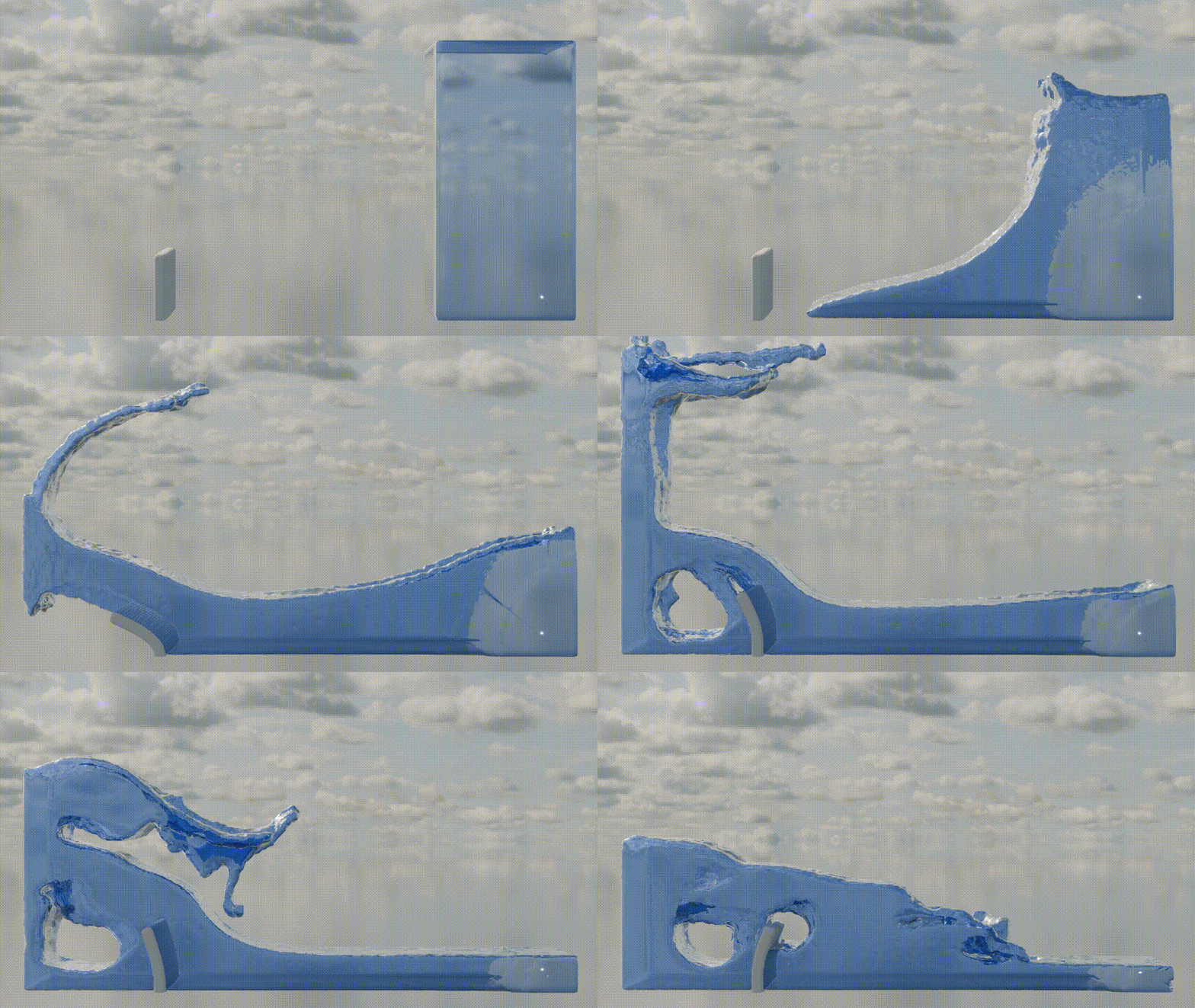
Forget about queues, job schedulers, or cluster configs. Just import, submit, and simulate.
Run DualSPHysics Across Different GPUs
In this tutorial, we’ll demonstrate how to use the Inductiva API to run DualSPHysics simulations on various GPU configurations.
To illustrate this, we’ll run a benchmark simulation based on the study presented in the paper A fluid–structure interaction model for free-surface flows and flexible structures using smoothed particle hydrodynamics on a GPU.
Among the simulations discussed, we focus on the 3-D dam break impacting an elastic plate scenario.

Simulation Overview
This simulation illustrates the classic dam break problem, where a column of water is suddenly released. What makes it unique is the presence of an elastic plate positioned at the opposite side of the domain, interacting dynamically with the fluid flow.
For more details, see section 4.5, 3-D dam break impacting an elastic plate, in the referenced paper.
Prerequisites
Download the DualSPHysics package
Download the required files from DualSPHysics_v5.4.2.zip here.
You will be working within this directory and writing the Inductiva Python script there.
Update the simulation script of the examples/flexstruc/01_DamBreak case
Before running the simulation, update the script located at: examples/flexstruc/01_DamBreak/xCaseDambreak3D_FSI_linux64_GPU.sh.
Make the following adjustments:
- Update the
dirbinvariable: Modify thexCaseDambreak3D_FSI_linux64_GPU.shscript to point to the correct binaries directory:export dirbin=/DualSPHysics/bin/linux/ - Remove user input prompt:
To enable automated execution, delete the final line in the script, which waits for user input:
read -n1 -r -p "Press any key to continue..." key
These modifications will prepare the script for seamless automated execution.
Running Your Simulation
Here is the code required to run a DualSPHysics simulation using the Inductiva API:
"""DualSPHysics example."""
import inductiva

# Allocate cloud machine on Google Cloud Platform
cloud_machine = inductiva.resources.MachineGroup(
    provider="GCP",
    machine_type="g2-standard-16",
    spot=True,
    data_disk_gb=200)

# Initialize the Simulator
dualsphysics = inductiva.simulators.DualSPHysics( \
    version="5.4.1")

# Run simulation
task = dualsphysics.run( \
    input_dir=input_dir,
    shell_script="xCaseDambreak3D_FSI_linux64_GPU.sh",
    # Convert VTK files to OBJ files for visualization
    vtk_to_obj=True,
    vtk_to_obj_vtk_dir="CaseDambreak3D_FSI_out/particles/",
    vtk_to_obj_vtk_prefix="PartFluid_",
    vtk_to_obj_particle_radius=0.002,
    vtk_to_obj_smoothing_length=2,
    vtk_to_obj_cube_size=1,
    on=cloud_machine)

# Wait for the simulation to finish and download the results
task.wait()
task.download_outputs()

cloud_machine.terminate()

task.print_summary()
This simulation runs in spot mode on a g2-standard-16 machine, featuring 16 virtual CPUs, 1 NVIDIA L4 GPU,
and a 200 GB data disk.
Note: Setting
spot=Trueenables the use of spot machines, which are available at substantial discounts. However, your simulation may be interrupted if the cloud provider reclaims the machine.
For visualization purposes, this script also optionally converts the simulation’s raw particle data (stored as .vtk files) into mesh format (.obj), making it compatible with common visualization tools. Check out this tutorial for more details.
When the simulation is complete, we terminate the machine, download the results and print a summary of the simulation as shown below.
Task status: Success

Timeline:
    Waiting for Input         at 26/05, 16:53:23      1.581 s
    In Queue                  at 26/05, 16:53:25      67.698 s
    Preparing to Compute      at 26/05, 16:54:32      9.148 s
    In Progress               at 26/05, 16:54:41      6861.774 s
        ├> 5862.434 s      bash xCaseDambreak3D_FSI_linux64_GPU.sh
        └> 999.117 s       splashsurf reconstruct CaseDambreak3D_FSI_out/particles//PartFluid_{}.vtk -r=0.002 -l=2 -c=1 -t=0.6 --subdomain-grid=on --mesh-cleanup=on --mesh-smoothing-weights=on --mesh-smoothing-iters=25 --normals=on --normals-smoothing-iters=10 -o CaseDambreak3D_FSI_out/particles//PartFluid__surface{}.obj
    Finalizing                at 26/05, 18:49:03      95.911 s
    Success                   at 26/05, 18:50:39

Data:
    Size of zipped output:    15.88 GB
    Size of unzipped output:  34.95 GB
    Number of output files:   1230

Total estimated cost (US$): 0.83 US$
    Estimated computation cost (US$): 0.82 US$
    Task orchestration fee (US$): 0.010 US$

Note: A per-run orchestration fee (0.010 US$) applies to tasks run from 01 Dec 2025, in addition to the computation costs.
Learn more about costs at: https://inductiva.ai/guides/how-it-works/basics/how-much-does-it-cost
As you can see in the "In Progress" line, the part of the timeline that represents the actual execution of the simulation, the core computation time of this simulation was approximately 1 hour and 37 minutes (5862 seconds).
Testing Across Different GPUs
As mentioned earlier, the simulation ran on an NVIDIA L4 GPU. To test it on other GPUs, simply change the machine_type parameter in the code to a2-highgpu-1g or a3-highgpu-1g. These machines come equipped with 1 NVIDIA A100 and 1 NVIDIA H100 GPU, respectively.
You also need to specify zone="europe-west4-b" when creating the machine, as the A100 and H100 GPUs are not yet available in our default zone.
Here are the results of running the same simulation on these machines:
| Machine Type | GPU | Execution Time | Estimated Cost (USD) |
|---|---|---|---|
| g2-standard-16 | NVIDIA L4 | 1h, 36 min | 0.66 |
| a2-highgpu-1g | NVIDIA A100 | 1h, 2 min | 0.61 |
| a3-highgpu-1g | NVIDIA H100 | 34 min, 33s | 1.55 |
Note: The times and costs listed above refer only to running the simulation and do not include the time required to convert VTK files to OBJ format. This conversion step is optional.
Check out our ParaView and Blender tutorials to learn how to visualize your simulation results.